Compare many cells
Sometimes you have to compare big tables and you need to do it fast. You can do it very easy and quick by using conditional formatting from excel. There are another ways too but I prefer this one because of it's simplicity and customization freedom/
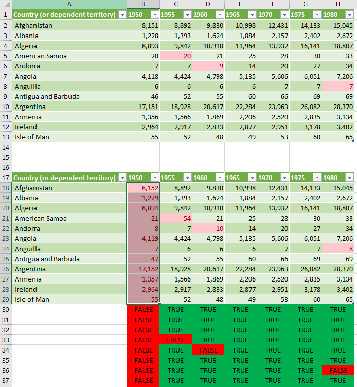
If you want to compare two big tables for changes - let says statistics or other data that changes on some time basis you could use these simple steps to make easier for you. On the picture below you can see sample tables that differ a little.
- first step is to create a check(in this case B30)
=B2=B18
-
second step is to add conditional formatting(you can check how here : Excel color rows based on a column value)
-
Go to manage rules
-
add new rule
-
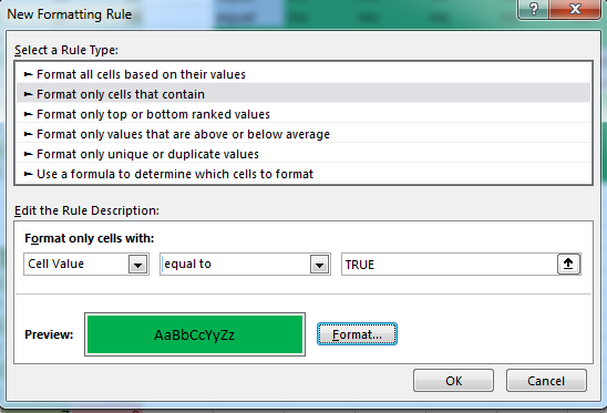
Format only cells that contain
-
Select equal
-
Write TRUE- or any other value that you want
-
Select desired format - in this case cell color green
-
Press OK
-
Next step is to repeat the process with equal to FALSE and format red cell
-
The last one - Expand selection to cover the whole table:
-
you can go to the left bottom corner of the cell and drag until the last column of the table (H)
-
then expand to all rows
Check increase, decrease or equal
A bit more tricky seems to be analyzing a trend: up, down or equal. Actually is very easy and close to the previous one. Below is shown the final result of it.
Here are the steps to follow:
- first step is to create a check cell(in this case J2) using this formula
=IF(B2=C2,"equal",IF(B2<C2,"inc","decr"))
feel free to customize it according your needs
-
second step is to add conditional formatting
-
Go to manage rules
-
add new rule
-
Format only cells that contain
-
Select equal
-
Write inc- or any other value that you want
-
Select desired format - in this case cell color green
-
Press OK
-
repeat for decr and equal
-
Expand selection to cover the whole table
That's it.


