In this post you can find how to build a simple machine learning model in Python. We will cover the basics of the ML model and how to build it quickly in a few lines of code.
Below you can find the full code of a machine learning model for classifying flowers based on their properties.
import seaborn as sns
from sklearn.model_selection import train_test_split
from sklearn.linear_model import LogisticRegression

iris = sns.load_dataset("iris")

X_train, X_test, y_train, y_test = train_test_split(iris.drop('species',axis=1), iris['species'], test_size=0.3, random_state=42)

model = LogisticRegression()
model.fit(X_train, y_train)

y_pred = model.predict(X_test)
Below you can find an explanation of the code and details.
Setup
We are using modules:
sklearn- for the ML moduleseaborn- for the training and testing dataset
We import the required modules and methods. Next we read the iris.csv dataset:
| sepal_length | sepal_width | petal_length | petal_width | species | |
|---|---|---|---|---|---|
| 0 | 5.1 | 3.5 | 1.4 | 0.2 | setosa |
| 1 | 4.9 | 3.0 | 1.4 | 0.2 | setosa |
| 2 | 4.7 | 3.2 | 1.3 | 0.2 | setosa |
| 3 | 4.6 | 3.1 | 1.5 | 0.2 | setosa |
| 4 | 5.0 | 3.6 | 1.4 | 0.2 | setosa |
The original dataset has 150 records.
Dataset preparation
ML models needs data for training which has:
- input
- sepal_length
- sepal_width
- petal_length
- petal_width
- output
- species
To build training and testing dataset we will split original dataset in 2 parts by:
input_data = iris.drop('species',axis=1)
output = iris['species']
X_train, X_test, y_train, y_test = train_test_split(input_data, output, test_size=0.3, random_state=42)
So we will have:
- X_train - 105 rows
- X_test - 45 rows
- y_train - 105 rows
- y_test - 45 rows
Example of X_train:
| sepal_length | sepal_width | petal_length | petal_width | |
|---|---|---|---|---|
| 81 | 5.5 | 2.4 | 3.7 | 1.0 |
| 133 | 6.3 | 2.8 | 5.1 | 1.5 |
| 137 | 6.4 | 3.1 | 5.5 | 1.8 |
| 75 | 6.6 | 3.0 | 4.4 | 1.4 |
| 109 | 7.2 | 3.6 | 6.1 | 2.5 |
and example of y_train:
81 	versicolor
133 	virginica
137 	virginica
75 	versicolor
109 	virginica
So we feed the model the properties of each flower and what is the name of it. The initial classification or labeling was done manually.
Training ML model
To train the model we will use LogisticRegression() and provide the training data:
model = LogisticRegression()
model.fit(X_train, y_train)
Testing model
Next we can test the machine learning model by:
y_pred = model.predict(X_test)
We can check the results:
array(['versicolor', 'setosa', 'virginica', 'versicolor'...
Now our machine learning model is able to classify flowers based on 4 inputs and return the species.
Verifying test results
To verify the test results we will use Pandas to compare the values:
(df.iloc[y_test.index]['species'] == y_test.values).value_counts()
which returns:
True	45
Name: species, dtype: int64
So we have 100% percent accuracy in prediction of iris species.
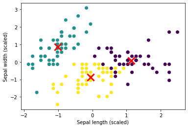
Visualizing data
We can use K-means to cluster data into groups and visualize it by:
- imports and dataset load
- build the K-means model
- use 3 clusters
- visualize the results
from sklearn.datasets import load_iris
from sklearn.preprocessing import StandardScaler
from sklearn.cluster import KMeans
import matplotlib.pyplot as plt

iris = load_iris()
X = iris.data

scaler = StandardScaler()
X_scaled = scaler.fit_transform(X)

kmeans = KMeans(n_clusters=3, random_state=42)
kmeans.fit(X_scaled)

plt.scatter(X_scaled[:, 0], X_scaled[:, 1], c=kmeans.labels_)
plt.scatter(kmeans.cluster_centers_[:, 0], kmeans.cluster_centers_[:, 1], marker='x', s=200, linewidths=3, color='r')
plt.xlabel('Sepal length (scaled)')
plt.ylabel('Sepal width (scaled)')
plt.show()
The results is below:


