Excel color rows based on a column value
Let imagine that you need to work with big excel table with information. You need to color rows based on some or several columns. This can be done very easy in several steps:
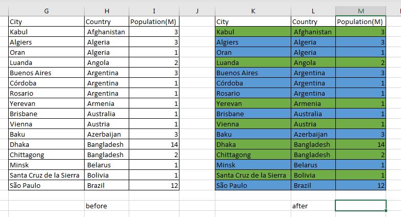
Final result
Conditional formatting rows in blue and green short
-
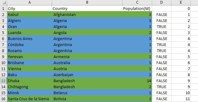
Add two columns at the end of sorted table(on B column). First is:
-
column D - D2 =B1=B2
-
column E - E1 = 0; E2 =IF(D2=TRUE;E2;E2+1)
-
conditional formatting
blue color
=NOT(MOD(INDIRECT(ADDRESS(ROW();5));2))
green color
=MOD(INDIRECT(ADDRESS(ROW();5));2)
Customisation
*In case that your column are different you need to change with the column that you will use for comparison:
=B1=B2
*For bigger table. 5 is the number of the column where you place : =IF(D2=TRUE;E2;E2+1). In this case is column E - so 5. If the column was D then the formula would be
=NOT(MOD(INDIRECT(ADDRESS(ROW();4));2))
Detailed explanation
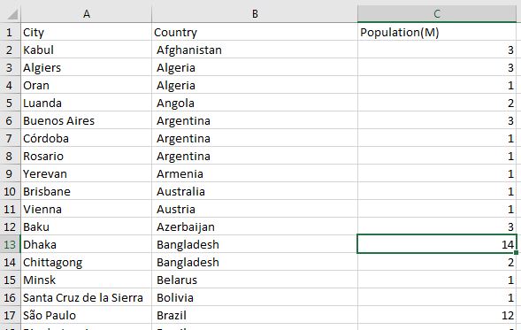
A table should be colored based on a column. Let have a table of cities per country and population. We want to alternate two colors based on the B column - country:
-
make a copy of your date and work on it - it will help you to verify that data is consistent after all operation or you can start again in case of mistake.
-
step one - sort table on column B
-
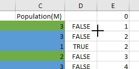
add new columns at the end of the table with formulas: D and E
-
start from D2- in the put: =B1=B2
-
E1 put 0, and in E2 put: =IF(D2=TRUE;E1;E1+1)
-
expand formulas up to the end of the table(you can click twice at left bottom corner of the cell)
-
click on a first row of the table
-
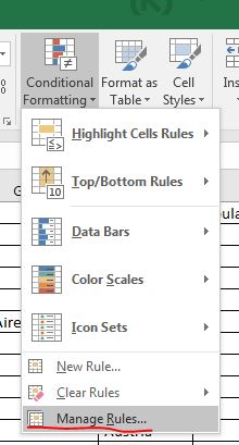
go to Conditional Formatting - > Manage Rules
-
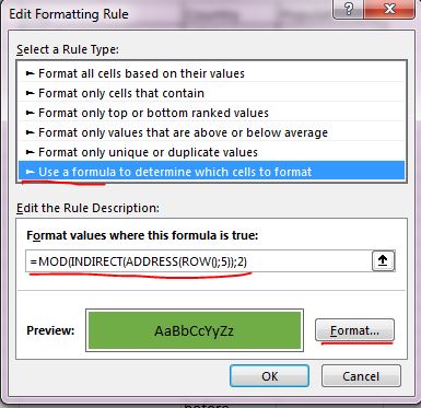
add a formula rule with the following formula:
=NOT(MOD(INDIRECT(ADDRESS(ROW();5));2))
- choose formatting for the cells by pressing Format
- you can change cell color, text color, and other settings of the cell
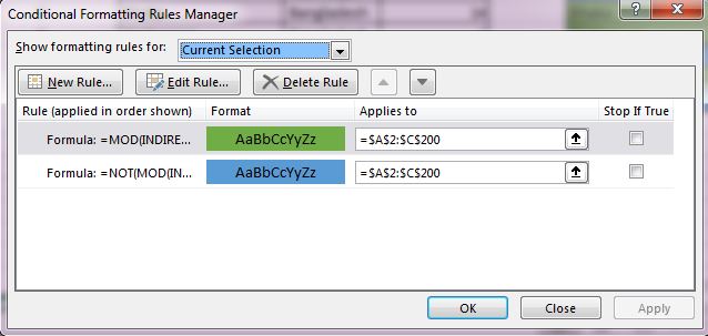
- select the range in Applies to
- =$A$2:$C$200
*repeat the above with:
green color =MOD(INDIRECT(ADDRESS(ROW();5));2)
- When you press Apply you should see immediately the results


