


In this article, you will find how to change the background color of a row based on a value in Google Sheets, Excel and Libre Office Calc. Also, you will learn how to use Excel formulas to get the value on a cell from a given row and use the same formula in Conditional Formatting.
You can find the complete example - all steps and data in these Google Sheet:
Alternate Row Color based on cell value
We have a table or range of data, and we want to change the background color of all cells in the row based on one of the cells from this row. Also, you want the color to change dynamically reflecting the data changes. You can find the result below:
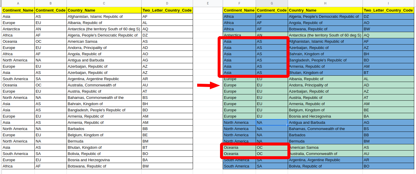
Data Source - list of countries by continent
Step 1: Sort data in Google Sheet
First we need to sort the data based on the column which is going to be used as a base for our color values - Continent_Code. This can be done by:
- Select the data Range -
A1:D26 - Data
- Sort Range
- Data has header row
- Sort by - Continent_Code
- Sort
Now data should be sorted and ready for our next step.
Step 2: Group rows based on value in a cell
This technique is exactly the same for both Excel and Google Sheets. Next we are going to group rows based on column Continent_Code and adding two helper columns. We are going to use column E and check is there a change for the values in Column Continent_Code - returning True and False.
So you need to use the formula in cell E2 and expand it until the end of the table(the result is True and False):
=B1=B2
The next is a numerical column which will start with 0 and increase the value by 1 for each group with this formula:
=IF(E2=TRUE,F1,F1+1)
Now we have the groups ready to be colored based on column F.
Step 3: Conditional Formatting on cell value
The final step is to add Conditional Formatting using a formula which will color different groups in two colors:
- even numbers in blue
- odd numbers in green
This can be done by:
- Select the table -
A1:D26 - Format
- Conditional Format
- From Format Rules
- Select Custom Formula is
- Enter the Formula:
=NOT(MOD(INDIRECT(ADDRESS(ROW();6));2))
- Change the formatting if needed
For the blue color repeat the previous steps but this time use the next formula:
=MOD(INDIRECT(ADDRESS(ROW();6));2)
and change the formatting to blue.
Tip: If you want to add similar rule like existing one - then you can select the existing rule and then press Add another rule.